Phylogeny
This page was produced as an assignment for Genetics 564 an undergraduate capstone course at UW-Madison.
Phylogenetics describes the analysis of the evolutionary history and relationships between species and populations using phylogenetic trees. Phylogenetics relies on phylogenetic inference methods to evaluate observable traits. Taxa lie on the tips of the branches of a phylogenetic tree. The point where two branches come together and meet is called a node, which represents the most recent common ancestor of the two connected branches. In Figure 1, Taxon A and Taxon B are connected at a node that represents their ancestor. Taxon C represents a distantly related group, in this case called an outgroup. Outgroups serve as a non-member reference for the analysis of a monophyletic clade, which is a group of organisms forming one clade, consisting of an ancestor and it's descendants. In Figure 1, Taxon A, Taxon B, and their common ancestral node form a monophyletic clade that Taxon C is the outgroup to. In molecular phylogenetics, sequence data is the observable trait used as input to describe the relatedness of taxa, individuals, or populations [1].
Using protein sequence data, I did a phylogenetic analysis of the ERCC6 protein.
Using protein sequence data, I did a phylogenetic analysis of the ERCC6 protein.
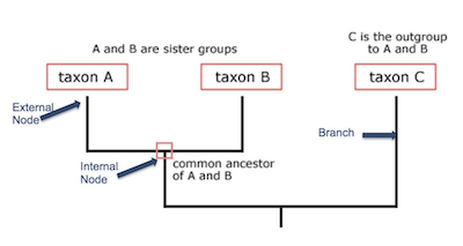
Figure 1. A simple phylogenetic tree.
ERCC6 Phylogenetics
In order to infer the relatedness of ERCC6 among many different species, I identified homologs of ERCC6 using Ensembl and constructed a FASTA formatted file containing the sequences for these homologs. Homologs from 16 species were chosen to represent diversity in the relatively well conserved ERCC6 gene. The 16 species chosen can be found on the Homology page of this website, and can also be identified, along with the sequence for their variant of ERCC6, in the FASTA formatted file below:
Using the FASTA formatted file of the 16 homologs as input data, I called on the program ClustalWOmega to analyze my data and generate phylogenetic trees. Below is a 111 amino acid screenshot of the sequence variation and conservation between the 16 taxa:
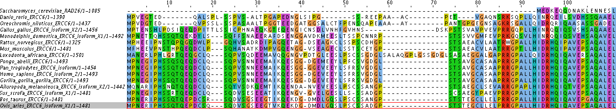
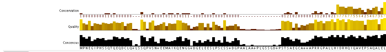
Figure 2. Data from my ClustalWOmega run.
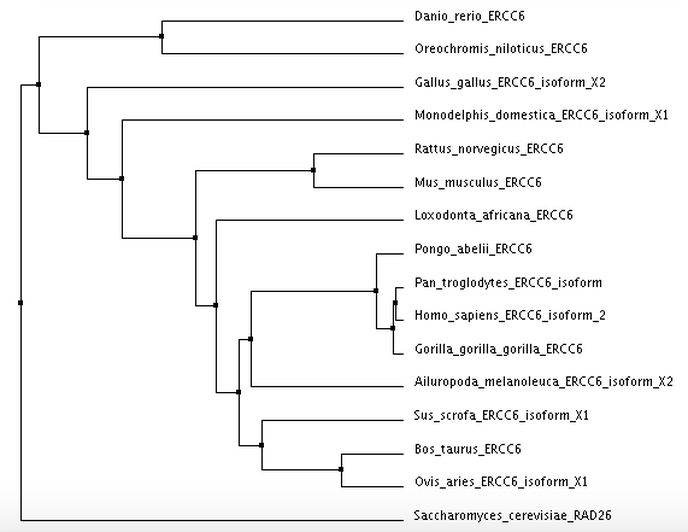
I calculated 4 trees using two separate distance matrix analysis methods: 2 using the BLOSUM62 matrix, and 2 using the Percent Identity matrix. Within each distance matrix method, I displayed one tree using the neighbor joining clustering method and another using the average distance clustering method.
|
Neighbor Joining
Neighbor joining clustering takes a distance matrix as an input and begins by constructing a star shaped tree, labeled (A) in Figure 3. The 'Q matrix' is calculated and two branches are joined to form a new node. This node becomes fixed, represented by the solid lines seen in node u in Figure 3. The distances from this node to the remaining taxa are calculated, and the branch with the shortest distance to the first node is joined, demonstrated by node v in part (C) of Figure 3. This process repeats until the tree has been resolved, as in part (E) of Figure 3 [2]. Average Distance Average distance clustering finds the lowest average amount of variation between all sequences and groups the sequences together based on their sequence similarity and distance. As the name implies, when two sequences are grouped together, their distance scores are averaged. In the example detailed in Figure 4, the table labeled (a) shows human with a distance score of 0 and chimpanzee with a distance score of 1.628. The difference between these two scores is the smallest possible difference out of the initial values given. Therefore, the human and chimpanzee scores are averaged, and the two taxa are clustered together, as shown in (b). In table (c), siamang and gibbon have the smallest difference between their values. Their scores are averaged, and the two taxa are grouped together, shown in (d). This process is repeated until all distance scores have been paired. At this point, the tree is resolved, shown in (h). |

Figure 3. The Neighbor Joining clustering method.
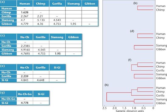
FIgure 4. A demonstration of the average distance clustering method. Note how after each pairing, the distances between the two species is calculated by averaging the scores of the two species.
|
Neighbor Joining using BLOSUM62
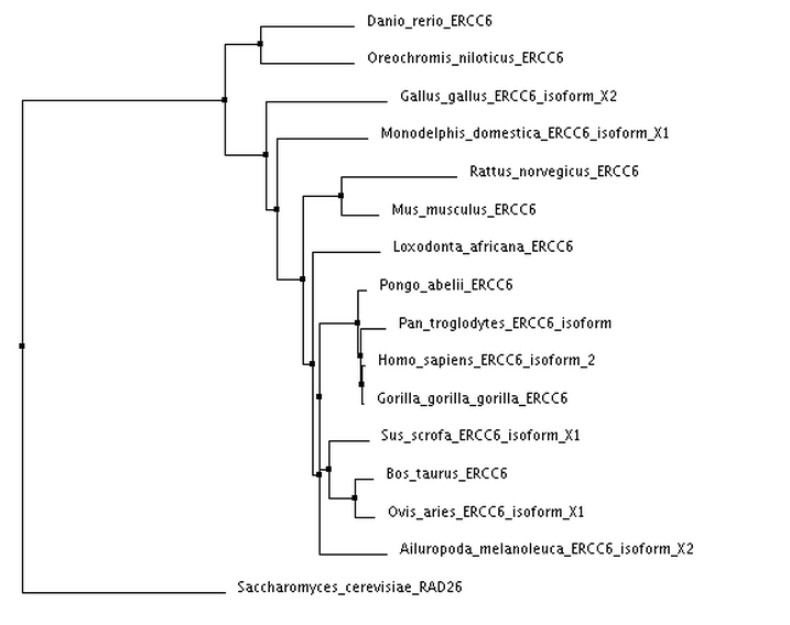
Neighbor Joining using Percent Identity
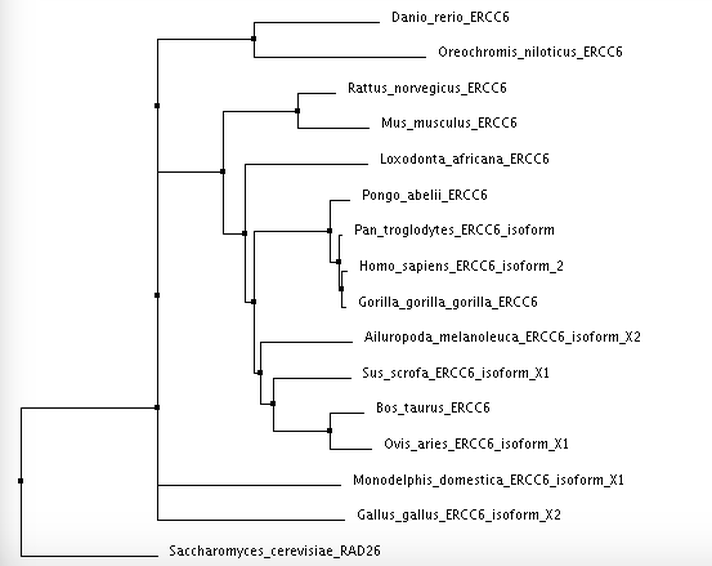
Average Distance using BLOSUM62
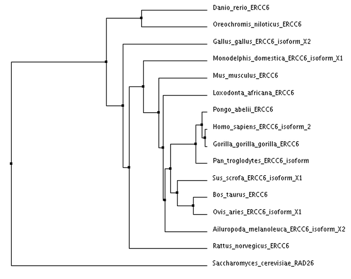
Average Distance using Percent Identity
References
[1] Yang, Z., Rannala, B. 2012. Molecular phylogenetics: principles and practice. Nat Rev Genet. 13(5):303-14. doi: 10.1038/nrg3186.
[2] Saitou, N., Nei, M. 1987. The neighbor-joining method: a new method for reconstructing phylogenetic trees. Molecular Biology and Evolution. 4(4): 406-425. https://doi.org/10.1093/oxfordjournals.molbev.a040454
Images and Videos
Phylogenetic tree diagram: http://study.com/academy/lesson/phylogenetic-tree-definition-types-quiz.html
Neighbor joining photo: https://en.wikipedia.org/wiki/Neighbor_joining
Average distance photo: http://bio3400.nicerweb.net/Locked/media/ch26/UPGMA.html
Tree photos are screenshots of the ClustalWOmega output.
Background photo modified from: www.pinterest.com/pin/313563192781815697/
This website was created for Genetics 564 by Zachary Beethem, an undergraduate genetics major at UW-Madison.
He can be reached via email: [email protected]
Date of last website update: April 2017
